Master the Timesheet Excel Formula for Accurate Calculations

The most important formula in your Excel timesheet is the one that calculates the total hours worked. It's a simple subtraction of the start time from the end time, but with one critical extra step: multiplying the result by 24. The formula looks like this: =(EndTime - StartTime) * 24.
Why the multiplication? Because that’s how you convert Excel’s internal time format into the decimal hours you actually need for payroll. Getting this right from the start saves you a world of headaches down the road.
Setting Up Your Timesheet for Flawless Formulas
Before you start plugging in formulas, you need a solid foundation. I’ve seen it a hundred times: a poorly structured spreadsheet is the number one reason formulas fail, spitting out frustrating #VALUE! errors and leading to inaccurate pay. Just taking a few minutes to set up clean, consistent columns is the secret to making everything work smoothly.
This isn't just about avoiding errors; it’s about ensuring your data is reliable from day one. When your data is clean, the formulas you build on top of it will be trustworthy and a whole lot easier to manage.
The Core Components of a Timesheet
A well-organized timesheet should break everything down into its own column. This simple structure makes your calculations straightforward and the whole sheet easy to read. For a basic setup, you’ll want columns for:
- Date: The day the work was done.
- Start Time: When the employee clocked in.
- End Time: When the employee clocked out.
- Break (in hours): The total time for any unpaid breaks.
- Total Hours: Where your formula will calculate the day's total.
Consistency is king here, especially with time entries. Stick to a standard format like HH:MM (e.g., 09:00 for 9 AM, 17:30 for 5:30 PM). If you start mixing formats, you're practically guaranteed to break your formulas.
Calculating Total Daily Hours
Now for the main event: calculating the hours worked in a day. A common mistake is just subtracting the start time from the end time. Excel will give you a result, sure, but it will be in its own special time format, not the decimal hours you need for payroll.
To get the right number, you have to multiply the result by 24. For example, if your start time is in cell B2 and the end time is in C2, your formula is: =(C2-B2)*24.
What about breaks? If you have a column for breaks (say, D2, with the break time entered as a decimal like 0.5 for 30 minutes), you just subtract that from the total: =(C2-B2)*24-D2.
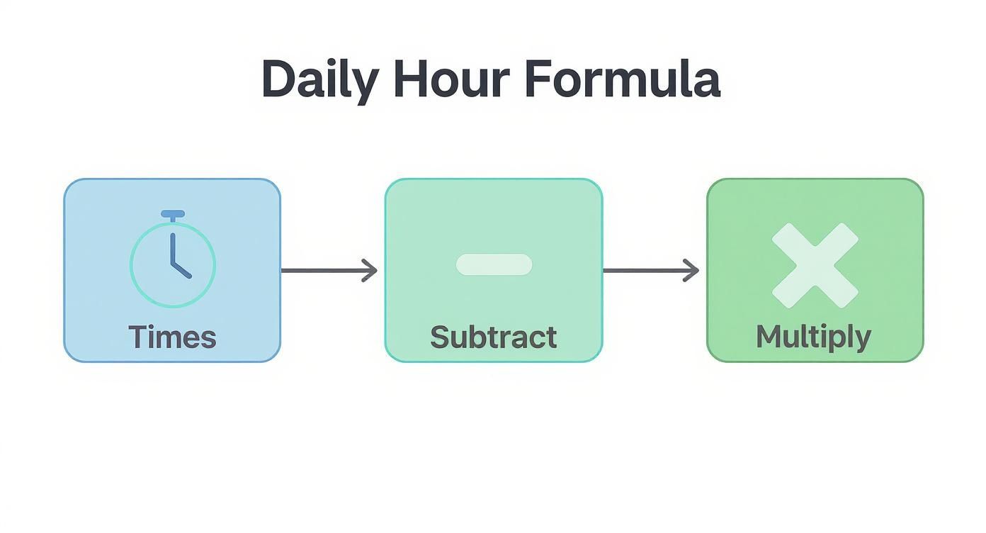
This simple process—subtracting times and then multiplying by 24—is the cornerstone of all your daily hour calculations.
To make this even clearer, here are the essential formulas you'll be using.
Essential Formulas for Daily Hour Calculation
| Scenario | Excel Formula Example | Explanation |
|---|---|---|
| Basic Hours Worked | =(C2-B2)*24 |
Calculates total hours by subtracting Start Time (B2) from End Time (C2) and converting to a decimal. |
| Hours Worked with Breaks | =(C2-B2)*24-D2 |
Same as above, but also subtracts the break duration (D2), which should be in decimal hours. |
| Hours with Breaks in Minutes | =((C2-B2)*24)-(D2/60) |
Use this if your breaks are entered in minutes (e.g., 30 for 30 minutes) to convert them to hours. |
These formulas are your starting point for building a reliable and accurate timesheet.
Key Takeaway: That
*24isn't just a suggestion; it's the non-negotiable step that turns Excel’s time value into a number you can use for wages, overtime, and project billing.
It’s no surprise that Excel is a powerhouse in the business world. With Microsoft Office 365 holding nearly 30% of the global market share, it’s the default tool for this kind of data management. In fact, Excel is the most popular tech skill listed in the United States, showing up in over 531,000 job postings.
Once you’ve got this fundamental formula down, you can start adding more features. A great next step is to build a holiday tracker Excel template that can work right alongside your timesheet. Getting this first piece right makes everything that follows so much easier.
Calculating Overtime and Variable Pay Rates
Once you've got the hang of tracking total daily hours, the next mountain to climb is payroll. This is where things get tricky, especially with overtime and different pay rates. Just adding up the hours won't cut it if you want to pay your team accurately and stay compliant. This is where a more sophisticated timesheet excel formula becomes your best friend, particularly when you use logical functions to automate the whole process.
The real workhorse for these calculations is the IF function. It’s a simple but powerful tool that lets Excel make a decision based on a condition you give it. For payroll, that condition is usually whether an employee has worked more than a set number of hours, like 40 in a week.
Segregating Regular and Overtime Hours
First things first, you need a cell that tallies up an employee's total weekly hours. A simple SUM function pointing to their daily totals will do the job. Let's say that grand total lives in cell F2.
With that total, you can now create two new columns: one for "Regular Hours" and another for "Overtime Hours." Splitting them up is key to applying the correct pay rates. The logic is simple: if the total is 40 hours or less, it's all regular. If it's more than 40, the first 40 are regular, and anything over that is overtime.
Here's how to turn that logic into formulas:
-
For Regular Hours: In your regular hours cell (let's say
G2), pop in this formula:=IF(F2>40, 40, F2)
This formula checks if the hours inF2are over 40. If they are, it puts40in the cell. If not, it just uses the actual number fromF2. -
For Overtime Hours: Next door, in the overtime cell (like
H2), use this:=IF(F2>40, F2-40, 0)
This runs the same check. If the total is over 40, it subtracts 40 to figure out the overtime. Otherwise, it simply returns0.
Just like that, you've cleanly split the hours, which makes calculating pay a whole lot easier.
Calculating Gross Pay with Overtime
Now that regular and overtime hours are in separate cells, figuring out gross pay is just some basic multiplication and addition. It's a good idea to put your standard and overtime pay rates in their own cells so you can update them easily. Imagine your regular rate is in cell J2 and the overtime rate (which is usually 1.5 times the regular) is in K2.
The formula for the total gross pay would be:=(G2 * J2) + (H2 * K2)
This formula just multiplies regular hours by the standard rate, does the same for overtime, and adds the two results together for the final weekly pay.
Pro Tip: Always use absolute references for your rate cells (e.g.,
$J$2and$K$2). This locks them in place. When you drag your formula down for other employees, it will keep pointing to the correct rates instead of shifting down with the formula.
Handling Variable Pay Rates for Different Roles
But what if you're managing a team where everyone has a different hourly rate? Or maybe you're tracking projects that are billed out at different rates. Typing these in manually is a recipe for mistakes and a huge time sink. This is where VLOOKUP really shines.
To start, you’ll need to set up a small reference table. You can stick it on another sheet or just in an unused part of your timesheet. This table needs at least two columns: one for the employee's name or ID, and one for their hourly rate.
Let's say your rate table is in the range M2:N10, with names in column M and rates in column N. If the employee's name for the row you're working on is in A2, your VLOOKUP formula would look like this:=VLOOKUP(A2, $M$2:$N$10, 2, FALSE)
This tells Excel to find the name from A2 in your rate table. Once it finds a match, it grabs the value from the second column (the pay rate). The FALSE at the end is super important—it makes sure you get an exact match, which is critical for accurate payroll.
Keeping up with legal requirements is also crucial. For example, in the United States, the federal minimum wage is $7.25 per hour, and overtime has to be paid at 1.5 times the regular rate. Smart timesheet templates often build these rules right into the formulas to ensure compliance.
By combining IF functions for overtime with VLOOKUP for variable rates, you can build a truly dynamic and automated payroll calculator in Excel. And remember, working with time in Excel often means dealing with conversions. If you need a refresher, our guide on converting minutes in decimals can be a lifesaver.
Solving Tricky Scenarios Like Night Shifts and Breaks

A standard 9-to-5 schedule is easy enough to calculate. But what happens when things get a little more complicated? If an employee works a night shift that crosses midnight, your simple subtraction formula will suddenly throw a fit. The end time (say, 2:00 AM) is technically "smaller" than the start time (10:00 PM), and Excel will return a negative number or an error.
This is a real headache for any business running 24/7 operations, from hospitals to security firms. The good news is that Excel has a clever function that fixes this problem beautifully, ensuring your timesheet can handle any schedule you throw at it.
Mastering the Overnight Shift with the MOD Function
The secret weapon for calculating hours across midnight is the MOD function. It might sound a bit technical—it returns the remainder of a division—but it's the perfect tool for handling time calculations that circle the clock.
When you subtract a start time from an earlier end time (like in a night shift), you get a negative value. The MOD function, when set up just right, flips this negative result into the positive duration you were actually looking for.
Let's assume the shift start time is in cell B2 and the end time is in C2. Here is the go-to formula for handling overnight shifts:
=MOD(C2-B2, 1) * 24
The beauty of this formula is that it works for every shift. If it's a normal day shift (e.g., 9:00 AM to 5:00 PM), C2-B2 is positive, and the formula calculates the hours correctly. If it’s an overnight shift (e.g., 10:00 PM to 6:00 AM), C2-B2 is negative, but the MOD function does its magic before the final multiplication by 24.
The Big Idea: That
MOD(..., 1)piece of the formula is what makes this work. It seamlessly handles both positive and negative time differences, giving you a robust, one-size-fits-all solution for any work schedule.
By using this formula, you build a truly flexible timesheet. No more manual fixes or clunky, error-prone IF statements just to deal with different shifts.
Effectively Managing Unpaid Breaks
Another area where mistakes often happen is accounting for unpaid breaks. Forgetting to subtract break time is one of the most common payroll errors out there, and it can easily lead to overpayments. You’ve got a couple of practical options for handling this in Excel.
The most direct method is to simply add a column for breaks. Employees can enter their break duration manually, which gives you a clear record. You can have them enter it in one of two ways.
-
Enter Breaks in Minutes: This is usually the most natural way for employees to think about it. If you go this route, you’ll just need to convert the minutes to hours in your formula. Say your total hours are calculated and the break time (in minutes) is in cell
D2. Your final formula would look like this:=(MOD(C2-B2, 1) * 24) - (D2/60) -
Enter Breaks as Decimals: Alternatively, you can have employees enter break time in a decimal format (e.g., 0.5 for 30 minutes or 1.0 for 60 minutes). This makes the final calculation a bit cleaner, since you can subtract the break value directly:
=(MOD(C2-B2, 1) * 24) - D2
Automating Standard Break Deductions
What if your company has a standard break policy, like a mandatory 30-minute unpaid lunch for any shift over six hours? You can automate this deduction completely. This takes the responsibility off your employees and guarantees consistency.
An IF function is perfect for this job. Let's stick with the policy of a 30-minute (0.5 hour) break for shifts longer than six hours. The formula would be:
=IF((MOD(C2-B2, 1) * 24) > 6, (MOD(C2-B2, 1) * 24) - 0.5, (MOD(C2-B2, 1) * 24))
Here’s a quick breakdown of what this formula is doing:
- First, it calculates the total hours worked using our trusty
MODfunction. - Next, the
IFfunction checks if that total is greater than 6. - If it is, the formula subtracts 0.5 hours from the total.
- If the shift is six hours or less, it leaves the total hours untouched.
This automated approach doesn't just save time; it enforces your company policy every single time, which can cut down on payroll disputes. By combining the MOD function for tricky shifts with smart break management, you can build a powerful and virtually error-proof timesheet.
Automating Weekly and Bi-Weekly Payroll Summaries
Calculating daily hours is a great first step, but the real magic happens when you automate your payroll summaries. Manually tallying up hours week after week isn't just a grind; it's practically an open invitation for costly mistakes to creep in.
The goal is to build a dynamic summary right into your timesheet. This way, you get an instant, at-a-glance view of total hours, overtime, and gross pay for any period. It’s about creating a template that updates itself as new time entries are added, cutting down on administrative work and giving you real confidence in your payroll accuracy. Functions like SUM and SUMIF are what turn your spreadsheet from a simple log into an intelligent assistant.
Building Your Summary Section with SUM
The most direct way to get a weekly total is with the good old SUM function. This is perfect for timesheets where each employee has their own tab or a clearly defined block of cells for the week.
Just pick a cell for your "Total Weekly Hours" and pop in a formula. For instance, if your daily totals are sitting in column F from row 2 down to row 8, you’d use this:
=SUM(F2:F8)
This simple timesheet excel formula just adds up everything in that range, giving you the weekly total. You can use the exact same logic to create summaries for regular hours, overtime hours, and gross pay by simply summing up their respective columns. It’s clean and effective.
Using SUMIF for Targeted Summaries
But what happens when you’ve got a single, running timesheet with multiple employees or pay periods all mixed together? That’s where SUMIF becomes your best friend. This function lets you add up numbers only if they meet a specific condition you set.
Imagine you want a separate table that calculates total hours for each person on your team. If employee names are in column A and their daily hours are in column F, the formula would look like this:
=SUMIF(A2:A100, "John Smith", F2:F100)
This formula scans the first 100 rows, finds every single entry for "John Smith," and adds up only their hours from column F. It’s a powerful way to pull specific data for employees, projects, or date ranges without having to manually filter or sort anything first.
Key Insight:
SUMIFtakes your timesheet to the next level by enabling conditional totals. Instead of just adding up everything in sight, you can tell Excel to sum hours only for a particular person or pay period. This makes your summary reports both dynamic and incredibly precise.
For businesses looking to integrate time tracking with other management tools, it's helpful to understand how different systems can work together. You can learn more about how to master time tracking tools with integration to make your processes even smoother.
While Excel formulas are robust, some businesses find that as they grow, transitioning from spreadsheets to specialized software for payroll and management becomes a necessary step.
To help you decide which approach is right for your current needs, here’s a quick comparison of the different ways you can summarize data in Excel.
Comparison of Summary Functions for Payroll Periods
The method you choose really depends on the complexity of your timesheet. For most small to mid-sized teams, SUM or SUMIF will handle everything you throw at them. But as your data grows, PivotTables can offer more powerful, interactive analysis.
| Method | Best For | Complexity | Key Advantage |
|---|---|---|---|
| SUM | Simple weekly or bi-weekly totals in a structured timesheet. | Low | Easy to implement for straightforward, periodic summaries. |
| SUMIF(S) | Summarizing hours for specific employees or projects from a mixed data set. | Medium | Offers conditional summing, making it highly flexible for detailed reports. |
| PivotTables | Creating interactive, in-depth summary reports from large datasets. | High | Allows for drag-and-drop analysis and multi-level data summaries. |
Ultimately, creating an automated summary section gives managers a clear, real-time overview of labor costs and employee hours without the headache of manual math. This doesn't just save a ton of time—it dramatically reduces the risk of human error in your payroll process.
Adding Professional Touches to Your Timesheet
A timesheet that gets the hours right is one thing. But a timesheet that’s easy to use, catches errors before they happen, and points you straight to the important numbers? That's a whole different level. These professional touches are what elevate a simple spreadsheet into a truly reliable business tool.
By building in features like data validation, conditional formatting, and cell protection, you’re not just making a fancier sheet. You're drastically improving its usability and the integrity of your data. These additions guide your team, slash the number of mistakes, and make the whole thing much faster to review at a glance.
Use Data Validation for Error-Free Entry
One of the most common headaches with any spreadsheet is a simple typo. A misspelled employee name or an inconsistent project title can instantly break summary formulas like SUMIF, sending you down a rabbit hole of frustrating troubleshooting. Data Validation is your secret weapon against this.
The idea is simple: create drop-down lists for any information that gets repeated. Think columns like "Employee Name," "Project," or "Task Type." This ensures every entry is perfectly consistent.
Here’s the quick way to set it up:
- First, create a master list of your items (like all employee names) in a separate tab or an out-of-the-way spot on your sheet.
- Select the cell or entire column where you want the drop-down to appear.
- Head to the Data tab on the ribbon and click Data Validation.
- In the pop-up, change the "Allow" dropdown to List.
- For the "Source," just select the range where you typed your master list. Click OK.
That's it. Now, users can only pick from your predefined list. Say goodbye to typos and hello to formulas that work every single time.
Highlight Key Information with Conditional Formatting
Conditional Formatting is an absolute game-changer. It’s an incredibly powerful feature that automatically changes how a cell looks based on what's inside it. This immediate visual feedback makes it effortless to spot critical information, like overtime hours or a missed clock-out.
You can use it to turn a wall of numbers into a dashboard that tells you a story.
A Few High-Impact Formatting Rules for Timesheets:
- Spotlight Overtime: Set a rule to turn any cell in the "Overtime Hours" column bright red if its value is greater than 0.
- Flag Missing Punches: Create a rule that highlights any blank "Clock In" or "Clock Out" cells, making it obvious where data is missing.
- Identify Long Shifts: Apply formatting to color-code any total daily hours that go over a certain threshold, like 10 hours, to keep an eye on potential burnout.
With a few simple rules, a manager can scan an entire weekly timesheet in seconds and immediately know what needs attention, without reading a single number. This visual layer makes approving timesheets ridiculously efficient.
Protect Your Formulas with Cell Protection
After you’ve dialed in your timesheet excel formula setup, the absolute last thing you need is for someone to accidentally type over a critical calculation and break the whole sheet. Excel’s cell protection feature is the perfect safeguard. It lets you lock down specific cells (like your formulas) while leaving others (like time entry cells) open for editing.
It's a straightforward two-step process. First, you tell Excel which cells people are allowed to edit, and then you lock the rest of the sheet down.
Putting Cell Protection in Place:
- Start by selecting all the cells your team needs to fill out—think clock-in/out times, break minutes, and project names.
- Right-click on your selection and choose Format Cells. Navigate to the Protection tab and uncheck the "Locked" box. Click OK.
- Now, go to the Review tab on the ribbon and click Protect Sheet.
- You can (and should) set a password, then just confirm the settings.
This simple action ensures your carefully crafted formulas stay safe and sound, while your employees can still enter their time without a hitch. These final touches are what make your spreadsheet a truly robust and dependable tool for managing time.
Got Questions? We’ve Got Answers.
When you start wrestling with Excel formulas for timesheets, you're bound to hit a few snags. It happens to everyone. Maybe you're getting a weird error message you can't decipher, or you're trying to nail down a specific payroll rule. Getting your timesheet to work perfectly often comes down to knowing how to handle these common hiccups.
Let's walk through a few of the most persistent questions that pop up and get them solved for good.
How Do I Fix The #### Error When Calculating Hours?
Ah, the classic wall of hash symbols (####). Seeing this is a rite of passage for any Excel user, and it almost always points to one of two things.
Most of the time, it's just a simple formatting issue: the column isn't wide enough to show the full value. The fix is a quick one. Just find the right edge of the column header and double-click it. Excel will automatically resize the column to fit the content.
The other culprit is a bit trickier and usually shows up when you’re summing hours that go past 24. For example, a total of 25 hours might display as "1:00" because Excel is thinking in terms of a 24-hour clock.
To sort this out, you need to give Excel a special instruction with a custom number format. Right-click the cell, choose Format Cells, and navigate to the Custom tab. In the type field, enter
[h]:mm. Those square brackets around thehare the key—they tell Excel you want to see total elapsed hours, not just the time of day. Your 25 hours will now show up correctly.
What Is The Best Way To Round Employee Hours?
Many companies round employee time to the nearest quarter-hour to make payroll a whole lot simpler. The cleanest, most reliable way to do this in Excel is with the MROUND function. It’s built specifically to round a number to the nearest multiple you give it.
For rounding to the nearest 15 minutes, this formula is your best friend:=MROUND(YourTimeValue*24, 0.25)/24
Here's a quick breakdown of what’s happening under the hood:
YourTimeValue*24converts Excel's time (which is a fraction of a day) into a simple decimal. So, 8:07 becomes 8.116.MROUND(..., 0.25)takes that number and rounds it to the nearest quarter (0.25). Our 8.116 becomes 8.25./24simply converts that decimal back into a time format Excel understands.
Using MROUND is a game-changer. It creates a fair and consistent system, which helps you avoid manual tweaks and potential payroll headaches down the line.
Can I Calculate Hours For Different Projects On One Timesheet?
You absolutely can, and it's a great way to see where your team's time is really going. The perfect tool for this job is the SUMIF function. It adds up numbers in one column but only if they meet a certain condition in another—like a project name. This is fantastic for tracking billable hours without juggling a mess of separate spreadsheets.
First, set up a "Project" column where employees can log what they're working on. A pro-tip here is to use Data Validation to create a dropdown list of project names. This keeps everything consistent and avoids typos that could break your formula.
Then, create a small summary table somewhere on your sheet with a list of your unique project names. In the cell next to a project name, pop in this formula:=SUMIF(ProjectColumnRange, ProjectNameCell, HoursColumnRange)
This tells Excel to scan your list of time entries, find every row that matches the project name you specified, and add the hours from those rows into a running total. It’s a beautifully simple way to get a clear, automated breakdown of project costs.
At DeskCove, we know that while Excel is a powerful tool, it has its limits, especially as your team grows. Our remote time tracking tool automates everything from capturing work hours to generating insightful reports on productivity. If you're ready to ditch the manual spreadsheet grind and simplify how you manage time, see what DeskCove can do for you.